Descriptive measures that indicate where the center or most typical value of a data set lies are called measures of central tendency or, more simply, measures of center. Measures of center are often called averages. The three most important measures of center are the mean, median, and mode. The mean and median apply only to quantitative data, whereas the mode can be used with either quantitative or qualitative (categorical) data.

The mean of a data set is the sum of the observations divided by the number of observations.  It's the familiar "average" you may have learned about.

The median of a data set is the number that divides the bottom 50% of the data from the top 50%. In order to find the median, arrange the data in increasing order. If the number of observations is odd, then the median is the observation exactly in the middle of the ordered list. If the number of observations is even, then the median is the mean of the two middle observations in the ordered list. In both cases, if we let n denote the number of observations, then the median is at position ^{(n + 1)}/₂ in the ordered list.

The mode of a data set is the value that appears most often.

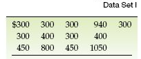
Example 1:

Professor Hassett spent one summer working for a small mathematical consulting firm. The firm employed a few senior consultants, who made between $ 800 and $ 1050 per week; a few junior consultants, who made between $ 400 and $ 450 per week; and several clerical workers, who made $ 300 per week. The firm required more employees during the first half of the summer than the second half. Tables 1 and 2 list typical weekly earnings for the two halves of the summer. Find the mean, mode, and the median of each of the two data sets.

Solution:

MEAN:

Data Set I has 13 observations. The sum of those observations is $ 6290, so

Similarly,

MEDIAN:

To find the median of Data Set I, wefirst arrange the data in increasing order:

300 300 300 300 300 300 400 400 450 450 800 940 1050  

The number of observations is 13, so ( n + 1)/ 2 = ( 13 + 1)/ 2 = 7. Consequently, the median is the seventh observation in the ordered list, which is 400

To find the median of Data Set II, we first arrange the data in increasing order: 300 300 300 300 300 400 400 450 940 1050 The number of observations is 10, so ( n + 1)/ 2 = ( 10 + 1)/ 2 = 5.5. Consequently, the median is halfway between the fifth and sixth observations in the ordered list, which is 350.

MODE:

In Data Set I, the value of $300 appears most often, so that is its mode.

In Data Set II, the most frequent value is also $300, so this again is the mode.

The figure below shows the relative positions of the mean and median for right-skewed, symmetric, and left- skewed distributions. Note that the mean is pulled in the direction of skewness, that is, in the direction of the extreme observations. For a right- skewed distribution, the mean is greater than the median; for a symmetric distribution, the mean and the median are equal; and, for a left-skewed distribution, the mean is less than the median. 

Population Mean and Sample Mean

Recall that a variable is a characteristic that varies from one person or thing to another and that values of a variable yield data. The values of a variable for an entire population are called population data; the values of a variable for a sample of the population are called sample data. The mean of population data is called the population mean or the mean of the variable; the mean of sample data is called a sample mean. The same terminology is used for the median and mode and, for that matter, any descrip-tive measure. Figure below shows the two ways in which the mean of a data set can be interpreted.

Possible interpretations for the mean of a data set

Summation Notation

In statistics, as in algebra, letters such as x, y, and z are used to denote variables. So, for instance, in a study of heights and weights of college students, we might let x denote the variable "height" and y denote the variable "weight". We can often use notation for variables, along with other mathematical notations, to express statistics definitions and formulas concisely. Of particular importance, in this regard, is summation notation.

Example 2:

The exam scores for the student are 88, 75, 95, and 100. (a.) Use mathematical notation to represent the individual exam scores. (b.) Use summation notation to express the sum of the four exam scores.

Solution: Let x denote the variable "exam score".

(a.) We use the symbol x_i ( read as x sub i) to represent the ith observation of the variable x. Thus, for the exam scores,

x₁ = score on Exam 1 = 88;

x₂ = score on Exam 2 = 75; 

x₃ = score on Exam 3 = 95;

x₄ = score on Exam 4 = 100.

More simply, we can just write x₁ = 88, x₂ = 75, x₃ = 95, and x₄ = 100. The numbers 1, 2, 3, and 4 written below the xs are called subscripts. Subscripts do not necessarily indicate order but, rather, provide a way of keeping the observations distinct.

(b.) We can use the notation in part ( a) to write the sum of the exam scores as x₁  + x₂ + x₃ + x₄.

Summation notation, which uses the uppercase Greek letter (sigma), provides a shorthand description for that sum. The letter corresponds to the uppercase English letter S and is used here as an abbreviation for the phrase the sum of. So, in place of x₁ + x₂ + x₃ +x_4, we can use summation notation, x_i , read as summation x sub "i" or the sum of the observations of the variable x. For the exam- score data,   x_i = x₁ + x₂ + x₃ +x₄ = 88 + 75 + 95 + 100 = 358

Interpretation:  The sum of the students four exam scores is 358 points.

Example 3:

Table above presents the arterial blood pressures, in millimeters of mercury ( mmHg), for a sample of 16 children of diabetic mothers. Determine the sample mean of these arterial blood pressures.

Solution: Let x denote the variable "arterial blood pressure". We want to find the mean, , of the 16 observations of x shown in Table above. The sum of those observations is  The sample size (or number of observations) is 16, so n = 16. Thus,

Interpretation: The mean arterial blood pressure of the sample of 16 children of diabetic mothers is 86.18 mm Hg.

EXERCISES:

Find the (a.) mean. (b.) median. (c.) mode(s). For the mean and the median, round each answer to one more decimal place than that used for the observations.

1. In a study of the effects of radiation on amphibian embryos, L. Licht recorded the time it took for a sample of seven different species of frogs and toads eggs to hatch. The following table shows the times to hatch, in days.

6

7

11

6

5

5

11